


| | | 2.7 Modelling of deposition |
Measurements of atmospheric deposition are generally expensive and time consuming and therefore sparse. In order to complement the monitoring and for other purposes as well atmospheric concentrations and depositions of nutrients are frequently calculated with the aid of atmospheric models.
What is the contribution from a source located at point A to the deposition of nutrients at point B?
What is the most feasible strategy in terms of economy for reducing the pollution e.g. with the goal of keeping the pollution and deposition below agreed limit values?
What will be the effect on local deposition of nutrients if a source is removed or added at a specific site?
Questions like these cannot be answered by measurements only. Full scale experiments are too expensive and involve a large risk of investing in the wrong solutions. Sensible use of suitable models provide the best answer in cases like these.
Procedure for construction of a model:
When the last step is completed the model is ready to be described in a programming language and run on a computer.
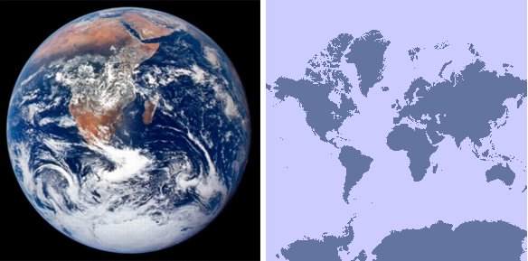
In order to construct a model describing transport and chemistry of certain species in the atmosphere, the ideal model domain would be the entire globe. However this is not very practical as the globe is spherical (see Figure 10) and the equations describing the physics are quite complicated in spherical co-ordinates.
The alternative is to select an area (a model domain) and make it flat, at least for the purpose of modelling it. This is illustrated in Figure 11 where the domain of a hemispheric air pollution model is presented. In this domain the surface of the majority of the Northern Hemisphere is projected on to a plane with the North Pole in the centre. This is called a polar stereographic projection, and for this particular example the projection is true at 60°north.
Independent of the projection, the domain of the model has to be discretized, horizontally as well as vertically. One way to carry out this discretisation is to divide the (3-D) model domain into boxes. How many boxes depends on what features the model should be able to describe. If -- for example -- the study is trying to quantify the nitrogen input into a coastal ecosystem, then the resolution has to reflect the size of this particular area as well as having a resolution that resolves the emission sources sufficiently to provide a realistic concentration and deposition distribution for the area.
In the case of the model domain presented in Figure 11 the horizontal domain is divided into 96 x 96 grid points, each with a size of 150 km x 150 km. This resolution is not high enough for studying nitrogen input to small water bodies, and the resolution is therefore increased over certain areas of the model domain. For this particular model an area over Europe is discretised with a 50 km x 50 km resolution and furthermore an area over Denmark and important surroundings is discretised with a resolution of 16.67 km x 16.67 km.
Other models have similar features in which the resolution is gradually increased over certain areas, thereby giving the possibility of `zooming' in on areas of interest. Due to the large amount of computer power needed for these kinds of models it is not possible just to increase the model resolution over the entire model domain. Due to the fast happening processes in the atmosphere it is necessary to have a quite large model domain in order to account for all the sources of nitrogen. If one imagines the concept of an airshed (similar to the concept of a watershed) then the airshed for a typical coastal area is many times larger than the watershed for the same area [364].
In order to model the processes in the atmosphere it is necessary to have a mathematical description of them. Considering chemical compounds in the atmosphere, the pathway to be described starts with the emission of the compounds, subsequent transport and dispersion by the wind, chemical transformation due to the influence of sunlight as well as mixing with other chemical components, and finally the deposition of the compound to the surface.
In mathematical terms this can be expressed as a set of partial differential equations (an example is given in Box 1), which in most cases (except for a few rather uninteresting ones) cannot be solved analytically. Instead the equations are solved numerically.
The mathematical description of the emission-transport-dispersion-chemistry-deposition pathway is in the Danish model DEHM-REGINA [89][164][163] given by the following set of differential equations:
For one specific location (grid point), the left hand side of the equation gives the change in concentration of chemical component i as a function of time. The first three terms on the right hand side of the equation describe the change in concentration due to transport by the wind (advection), the next three terms describe the change in concentration due to dispersion and the last three terms describe the change due to emissions, wet deposition and chemical reactions respectively. The process of dry deposition is described by the vertical dispersion term, where dry deposition is the lower boundary condition.
In order to solve the set of equations it is customary to perform a so-called splitting and divide the equation into submodels, i.e. first calculate the change in concentration due to advection, then the change in concentration due to dispersion and finally the change in concentration due to chemistry, emissions and wet deposition. Each of these so-called sub-models have different mathematical and numerical properties. In order to optimize the accuracy and stability of the solution it is therefore custom to apply different numerical solution techniques for the different parts of the equation (the different sub-models). However, such a procedure needs a careful analysis in order to avoid numerical errors especially when a splitting is performed for processes taking place on similar timescales.
The set of equations depicted in Box 1 has to be solved for every grid box in the model domain, for every time step of the model run. Taken the model with the domain in Figure 11 as an example there are 96 by 96 by 20 grid boxes in the model. Furthermore there are 60 chemical species in the model giving a total of 11,059,200 equations with the same amount of unknowns to be solved at each time step. A time step in an atmospheric transport chemistry model typically has a value around 500 seconds depending on the time of the day (many chemical reactions depend on the amount of sunlight available) and this gives approximately 5400 time steps to be carried out to complete calculations for one month. In total that means that 59,241,922,560 equations have to be solved, each involving many floating points operations (flops). Atmospheric transport-chemistry models are therefore typically operated on large workstations or computer clusters, rather than on ordinary personal computers.
Once the solution technique for the equations is in place, several kinds of input data are required for the model calculations:
Meteorological data may be obtained from many different sources, however the use of output from numerical weather prediction (NWP) models is becoming more and more frequent. This type of data should be 3-D in order to describe the three-dimensional transport in the atmosphere. The temporal resolution of data sets like these are typically a couple of hours and the meteorological variables are then interpolated in the air pollution model in order to get meteorological fields for every time step. It is possible to save data from the NWP model with a higher frequency, however the disc space needed for storage usually sets the limit. A way to work around this problem is to run the NWP coupled together with the air pollution model, thereby calculating the meteorological variables everytime the air pollution model is run. This in turn gives rise to a problem concerning computation time, especially if the model has to be applied for various scenarios.
In the DEHM-REGINA model mentioned previously, the meteorological input consists of results from the NWP MM5 (Mesoscale Meteorological Model, Version 5, [180]). An example of output for the hemispheric model domain (presented in Figure 11) is given in Figure 12.

Emission data for all the primary components included in the model are also necessary. The data should be gridded and as many of the sources as possible should be included. Emission data are typically obtained as yearly totals, or in some cases as monthly totals. The seasonal as well as the day to day variation can however be quite strong, and if possible data sets with (at least) a seasonal variation should be applied.
Alternatively parameterisations of the temporal variations can be used. An example of a parameterisation of the temporal variation in NH3 emissions is presented in Figure 13. The day to day changes in emission are in this case based on information concerning agricultural practise and the variations within the day are parameterised according to meteorological factors such as temperature and wind speed [5]. The result is a significant spring peak in the emissions.
Figure 13 presents the emissions calculated for the years 1999, 2000 and 2001 for a specific site in Denmark (the measurement station Tange). The emission peaks are slightly shifted from year to year as a result of temperature distribution differences between the years (in a cold spring the emission peak will be located later than in a relatively warm spring period).
In Figure 14 are shown to sets of time series of concentrations. Each set consists of one curve presenting measured concentrations at Tange and one curve presenting concentrations for Tange calculated with an air pollution model. The emission data input for the model results presented to the left in the Figure contain no information considering the temporal variation, whereas the emission data input for the time series presented in the right part of the Figure includes the parameterisation of the temporal variation presented in Figure 14. It is clear from the figures that for the component NH3 it is very important to describe the temporal variations of the emissions in the model in order to be able to reproduce measured concentrations [5].
Considering again the DEHM-REGINA model as an example, there are 16 different chemical components which are primary. Emission data sets for these components are derived from a combination of hemispheric and European data sets and an example of the ammonia (NH3) emissions for different horizontal resolutions are given in Figure 15.
The dry deposition of pollutants and nutrients is dependent on the composition of the surface and therefore it is necessary also to include data describing the surface characteristics. In this kind of data sets the surface is classified into a number of different categories like e.g. forest, crop land, water areas etc. An example of a land use data set for one specific category is presented in Figure 16.
The atmosphere is a chemically dynamical environment and starting a model run with concentrations of the different chemical components equal to zero will result in a system which requires a very long spin-up time in terms of the modelled time period to become balanced (several years). If instead the initial conditions consist of a set of background concentrations for the different chemical components, the spin-up time can be reduced to a couple of months calculated (again in terms of modelled time period). During the model run boundary conditions are needed in order to describe what is the concentration of the air flowing in from outside the model domain at the lateral boundaries as well as at the top of the domain.
It is very important that the resolution in the input data is at least as high as the resolution of the model domain. If the resolution in the input data is coarser than the resolution of the model, then the amount of information needed for fully exploiting the capacity of the model with its given resolution is too small.
Model results are obviously only useful if the models are capable of representing the actual situation. That is, if the model results comply with the results obtained from measurements. In order to evaluate the performance of an air pollution model it is therefore common to carry out a validation with measurements of air pollutant concentrations and depositions. This is done by comparing e.g. calculated and measured mean concentrations or accumulated depositions on monthly (mainly depositions), daily or hourly basis for as many measurement stations as possible.
To determine how the model is performing in general the concentrations from all available measurement stations can be compared with calculated values in a so-called scatter plot (see Figure 17). If the model is perfect for all the different areas represented by different measurement stations, then all the points in the scatter plot will lie on the 1:1 line. Deviations from this line is an indication of the concentrations being either over- or underestimated by the model. In order to determine how well the performance of the model is, several statistical parameters are calculated on the basis of the data set. These parameters are also used in e.g. sensitivity analyses of different model configurations.
In order to determine when and where the over- or underestimated values are obtained the calculated and measured values can be compared in time series (see Figure 18). The time series can be investigated for just one measurement station in order to understand the behaviour of the model in the particular region where the station is located, or it can be investigated for the mean value of all the measurements obtained at the different stations.
One of the advantages of applying a model is that the deposition to e.g. an entire area can be assessed, even for areas that are not accessible for performing measurements. An example of an atmospheric transport-chemistry model that has been extensively used in this context is the Atmospheric Chemistry and Deposition model (ACDEP; [231]). This model is applied in the Danish Background Monitoring Programme for calculating surface concentrations and depositions of nitrogen and sulphur to Danish land and sea areas. The irregular model domain covers the Danish national territory and the horizontal resolution of the model is 30 km. An example of calculated nitrogen depositions for the year 2002 is presented in Figure 19. It is important to note that the dry deposition velocity is different for land and sea surfaces and therefore there are two different deposition maps, one for land, and one for the marine areas, lakes and streams.
The ACDEP model has also been utilised in other research projects where larger water bodies have been the focal point. Examples are calculations for the Baltic Sea area [231] and the North Sea area [230].
Considering the calculations for the Baltic Sea, the nitrogen deposition was calculated with a horizontal model resolution of 30 km to the entire Baltic Sea area, and furthermore surface concentrations at 16 measurement stations located in Denmark, Sweden, Germany, Finland, Poland, Estonia, Latvia and Lithuania were calculated in order to compare the calculated concentrations with measurements in the vicinity of the Baltic Sea.
An example of the computed total atmospheric nitrogen deposition for the year 1999 is presented in Figure 20. The deposition has a pronounced south-north gradient with depositions in the range from 1000 kg N km-2 in the south to 200 kg N km-2 in the north. This gradient is due to transport from the areas with high emission densities in the northern part of the European continent. These results are consistent with results from other air pollution models [230].
The results from the ACDEP model studies on the deposition to the Baltic Sea region, supports the generally accepted fact that episodes of high atmospheric nitrogen deposition are the result of precipitation events. Depositions may be somewhat elevated close to the coast when transport from nearby agricultural activities lead to high ammonia concentrations. However, the resulting dry deposition is considerably smaller than what is observed from rain out of ammonium and nitrate in particulate form.
In Figure 21 is shown a simulation of an event with high local wet deposition of atmospheric nitrogen in a belt from the coast of Poland and out to Gotland in the Baltic Sea. The simulation is performed with the ACDEP model. The episode took place on July 26, 2002 and the results in the figure are given in the form of daily mean values (for the concentrations) and daily total values (for the precipitation and deposition). In Figure 21 is shown the precipitation in mm (upper left), the concentration of ammonia in µg N m-3 (upper right), the concentration of particulate ammonium in µg N m-3 (lower left) and the total nitrogen deposition in Tonnes N km-2 (lower right).
As described in Section the dry deposition is related to the atmospheric concentrations of gas-phase ammonia, whereas the wet deposition is related to the concentrations of particulate-phase ammonium. When the precipitation plot (the upper left part of the figure) is compared with the ammonium concentration plot (lower left part of the figure) and the total deposition plot (lower right part of the figure) it can be seen that high concentrations of ammonium in the southwestern part of the Baltic combined with moderate precipitation amounts in the same region produce high amounts of deposition. Likewise moderate concentrations of ammonium in the Gulf of Riga, the Gulf of Finland and the northern part of the Gulf of Bothnia as well as off the coast of Latvia and Lithuania combined with high amounts of precipitation in these areas also produce peaks in the atmospheric deposition of nitrogen.
Another example of atmospheric deposition calculated with an air pollution model is presented in Figure 22 showing the atmospheric deposition to the North Sea calculated with the ACDEP model [231]. The depositions are seen to vary between 0.3 to more than 3 tonnes N km-2. Smallest values are found in the northern part of the North Sea, that is far from the large source areas in the northern part of the European continent. Largest deposition densities are found in the southern part and especially at the coastline of France, Germany, Belgium and the Netherlands.
| | | 2.7 Modelling of deposition |