


| | | 8.5 Algorithms of primary production versus vertical carbon export |
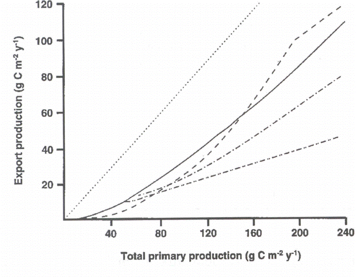
An overview on algorithms predicting export production on the base of total primary production in marine environments on an annual scale has been presented by [487][489] (Figure 4). Significant variability with regard to the PE versus PT relationship was detected. What algorithm should be selected for a global or coastal eutrophication carbon flux model? Obviously, there is no universal algorithm that would fit all ecosystems. Does the variability of the algorithms reflect real difference in the PE vs. PT relationships in the various ecosystems from which they were derived (Figure 5B)? If so, then different algorithms should be applied in different regions.
In particular data from the boreal coastal zone from the North Atlantic were investigated. The data used was mainly selected from simultaneous, time-integrated measurements derived over intervals covering most of the productive season (>6 months). Through a regression analysis PE was positively and nonlinearly correlated with total production PT (Figure 5A). Best fit (r2 = 0.94) was found by a power model calculated by the equation:
PE = 0.049 PT1.41
The <e> ratio was also calculated and both <e> and PR were found to be positively, nonlinearly correlated with PT. The upper limit for <f> was calculated to be about 0.5 in boreal coastal environments, i.e. at most about 50% of PT may be exported through sedimentation to below the euphotic zone. The curvilinear nature of the relationship implies that vertical export of biogenic matter increases significantly more than total primary production.
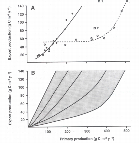
The results of the model of Aksnes & Wassmann [2] indicate that domination by copepods in the marine and cladocerans in lakes can give rise to very different relationships between primary versus export production (Figure 5A). Meso-zooplankton species composition obviously influences the pelagic-benthic coupling: for example, copepods and cladocerans have different reproductive strategies (hence different grazing pressure), and cladocerans do not produce distinct faecal pellets. A comparison of retention and export food chains, and vertical flux in lakes dominated by copepods (e.g. Lake Baikal) or marine environments strongly influenced by cladocerans (e.g. the eastern Baltic Sea), would be advantageous to analyse in greater detail the contrasting scenarios of copepod and cladoceran dominance for pelagic-benthic coupling.
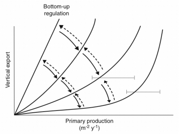
In case the algorithms depicted in Figure 5A are truly predicting annual PE on the base of PT, why are there significant differences? In the case of subalpine lakes and boreal coastal areas we have already recognised that differences in the zooplankton community species composition result in the observed variance. The question can be raised if the results presented in Figures 4 and 6 suggest that various types of top-down regulation are the base for the observed variability? The few data which do exist from non-boreal environments outside the North Atlantic suggest that coastal areas and tropical bays in the North Pacific Ocean experience more efficient retention in the upper layers and less vertical export (Figure 5A). This interpretation is in consistency with the notion that tropical environments are characterised by effective retention food chains. This may also be true for the North Pacific Ocean where at least the open ocean is characterised by extensive micro-zooplankton grazing which prevents major accumulation of phytoplankton biomass [165][110]. PE as a function of PT in miscellaneous ecosystems with different production, recycling and export regimes could fall onto a suite of lines falling between maximum export (steep angle, straight line = bottom-up regulation) and high retention (flat angle, curved line = top-down regulation) efficiencies (Figure 6). The balance between bottom-up and top-down regulation shapes the curvilinear nature of the PT vs. PE relationship. Not only PT varies as a function of climate variability and eutrophication, also the PT/PE ratio is not constant, but varies in accordance with the composition and dynamics of the heterotrophic plankton community. `The' PT vs. PE relationship does that not exist.
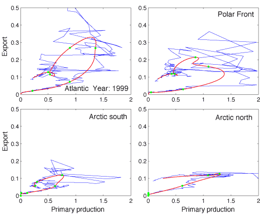
On a daily scale the PT vs. PE relationship is characterised by irregularities (Figure 7). Primary production varies greatly between days and contributes to in different degrees to the suspended pool of biogenic matter (a function of total production, the f-ratio, grazing etc.) that may sink. Although short-term variability in vertical flux takes place, that of primary production is greater. The phase plot in Figure 7 illustrates the spiky nature of primary production as compared to the buffered rates of vertical export. The 5 days running average plot indicates the loop-type relationship between daily PT and PE, as predicted by Wassmann [490]. Increased bottom-up regulation by eutrophication will increase the `loopy' nature of the PT vs. PE relationship. In contrast, increased top-down regulation will decrease the loop size. Increased top-down regulation will eventually force the loop onto a retention line and remove excessive vertical export.
| | | 8.5 Algorithms of primary production versus vertical carbon export |