


| | | 2.3 Transport |
The driving force of the atmosphere described by the meteorology is responsible for the transport of nutrients (and pollutants) in the troposphere. Pressure and temperature gradients make the air masses move and the result is that the nutrients (in gaseous and particulate form) are moved along with the air.
The region of the atmosphere governing transport and dispersion of the majority of the pollutants is the planetary boundary layer. This layer is defined as the layer where the wind structure is influenced by the surface of the Earth.
The wind transports the air masses around, however, the wind is, through the mechanical formation of turbulence, also responsible for a significant part of the mixing of the pollutants in the air.
There are two types of turbulence; mechanical and convective. Mechanical turbulence, characterised by small eddies close to the surface, is thus a result of the wind dragging over the surface. Smooth surfaces like fields of grass or calm water surfaces produce little mechanical turbulence, whereas rough surfaces like forests or buildings can result in the production of large amounts of mechanical turbulence. Convective turbulence, characterised by large eddies with a long lifetime, is the result of the sun heating the surface, which then in turn heats the air mass just above the surface. This heated air mass then rises because of its temperature being higher than the temperature of the surrounding air -- so-called bouyancy -- and the result is turbulence.
Several other meteorological factors may affect the concentration of pollutants in the air:
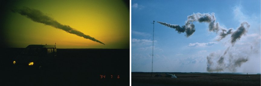
The atmospheric conditions may be divided into three classes in terms of stability: neutral, stable and unstable conditions. These three categories are characterised by the following:
Examples of the behaviour of a plume from a chimney under stable and unstable conditions are shown in Figure 3.
The height of the planetary boundary layer varies with the atmospheric stability and this is important for the concentrations of pollutants in the air because the majority of the pollutant mass typically is confined within this layer. During nighttime when conditions in most cases are stable, the planetary boundary layer is shallow, down to 20-50 meters and the surface concentration of pollutants can therefore be quite high, especially close to emission sources that are active during the night. Under unstable conditions the planetary boundary layer can be as high as 2 kilometers and pollutants are in this case distributed in the air column mainly by convective turbulence. In the vicinity of the top of the boundary layer, the horizontal winds are typically stronger and the pollutants that end up at these higher levels may be transported far away from the emission sources. In neutral conditions emitted pollutants are quickly mixed in the air by mechanical turbulence and the surface concentration is not particularly high. During neutral conditions the strong horizontal wind speeds can transport pollutants across large distances.
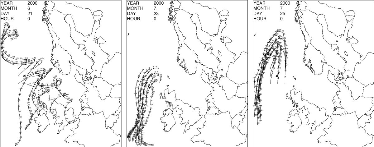
It is important to realise that pollutants emitted at the surface at one point may travel to a completely different location before they are deposited. A typical method to study the movement of air masses is to calculate so-called trajectories based on the wind speed and direction. Trajectories can be calculated forward as well as backward in time. Forward trajectories are typically used in connection with the calculation of pollutant distribution from accidental releases where the emission source is single and strong, whereas the backward trajectories are typically used for modelling air pollution from multiple distributed emission sources.
The procedure for calculating backward trajectories is to choose a starting point and then calculate back in time according to the direction and speed of the wind. In order to study the sensitivity of the trajectories to the choice of starting point several trajectories can be calculated with pertubed starting points. An example of a such a sensitivity investigation is given in Figure 4. In the left and center part of the figures it is seen that even though the wind may come from one direction at the surface, this does not necessarily mean that it is the direction the air mass is coming from originally. In the right hand part of the figure is given an example where 150 km difference in starting points for the trajectories results in a completely different origin of the air mass.
Another method for testing the accuracy of calculated trajectories is to release large numbers of balloons with tracking equipment and then evaluate the calculated trajectories with the observations. An example of such an evaluation can be found in Stohl [444]: a review of trajectory application.
| | | 2.3 Transport |